1/1/2018

根据与基因的相对位置，lncRNA可以分为Intergenic LncRNAs(lincRNA), Bidirectional LncRNAs, Intronic LncRNAs, Antisense LncRNAs, Sense-overlapping LncRNAs五类，每类详细定义规则如下：

定义

ref: https://www.arraystar.com/reviews/v30-lncrna-classification/

1. Intergenic LncRNAs

   

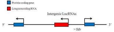
   Intergenic LncRNAs are long non-coding RNAs which locate between annotated protein-coding genes and are at least 1 kb away from the nearest protein-coding genes. They are named according to their 3-protein-coding genes nearby. Gene expression patterns have implicated these LincRNAs in diverse biological processes, including cell-cycle regulation, immune surveillance and embryonic stem cell pluripotency. LincRNAs collaborate with chromatin modifying protein (PRC2, CoREST and SCMX) to regulate gene expression at specific loci.

2. Bidirectional LncRNAs

   

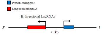
   A Bidirectional LncRNA is oriented head to head with a protein-coding gene within 1kb. A Bidirectional LncRNA transcript exhibits a similar expression pattern to its protein-coding counterpart which suggests that they may be subject to share regulatory pressures. However, the discordant expression relationships between bidirectional LncRNAs and protein coding gene pairs have also been found, challenging the assertion that LncRNA transcription occurs solely to “open” chromatin to promote the expression of neighboring coding genes.

3. Intronic LncRNAs

   

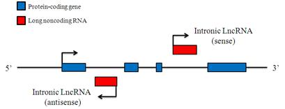
   Intronic LncRNAs are RNA molecules that overlap with the intron of annotated coding genes in either sense or antisense orientation. Most of the Intronic LncRNAs have the same tissue expression patterns as the corresponding coding genes, and may stabilize protein-coding transcripts or regulate their alternative splicing.

4. Antisense LncRNAs

   

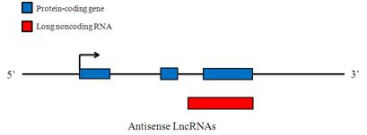
   Antisense LncRNAs are RNA molecules that are transcribed from the antisense strand and overlap in part with well-defined spliced sense or intronless sense RNAs. Antisense-overlapping LncRNAs have a tendency to undergo fewer splicing events and typically show lower abundance than sense transcripts. The basal expression levels of antisense-overlapping LncRNAs and sense mRNAs in different tissues and cell lines can be either positively or negatively regulated. Antisense-overlapping LncRNAs are frequently functional and use diverse transcriptional and post-transcriptional gene regulatory mechanisms to carry out a wide variety of biological roles.

5. Sense-overlapping LncRNAs

   

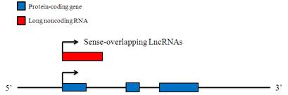
   These LncRNAs can be considered transcript variants of protein-coding mRNAs, as they overlap with a known annotated gene on the same genomic strand. The majority of these LncRNAs lack substantial open reading frames (ORFs) for protein translation, while others contain an open reading frame that shares the same start codon as a protein-coding transcript for that gene, but unlikely encode a protein for several reasons, including non-sense mediated decay (NMD) issues that limits the translation of mRNAs with premature termination stop codons and trigger NMD-mediated destruction of the mRNA, or an upstream alternative open reading frame which inhibits the translation of the predicted ORF.

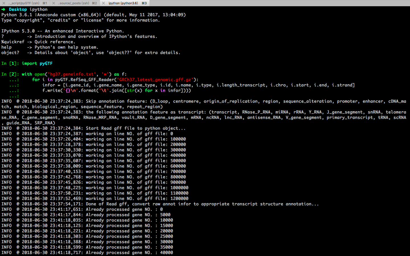
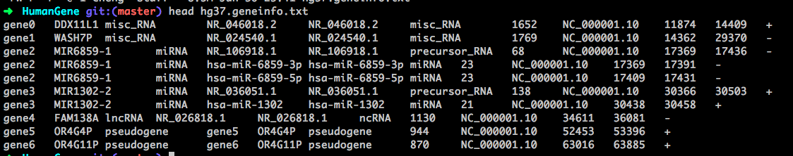
实现

1
2
3
4
5
6
7
8
9
10
11
12
13
14
15
16
17
18
19
20
21
22
23
24
25
26
27
28
29
30
31
32
33
34
35
36
37
38
39
40
41
42
43

# step0 prepare
awk -F "\t" 'BEGIN{OFS="\t"}{if ($3=="transcript") {print $1,$4,$5,$9,$7}}' lnc.gtf | sed -e 's/gene_id.*transcript_id "//g' -e 's/".*\t/\t.\t/g' >lnc.transcript.bed
awk -F "\t" 'BEGIN{OFS="\t"}{if ($3=="transcript") {print $1,$4,$5,$9,$7}}' mRNA.gtf | sed -e 's/gene_id.*transcript_id "//g' -e 's/".*\t/\t.\t/g' >mRNA.transcript.bed
awk -F "\t" 'BEGIN{OFS="\t"}{if ($3=="exon") {print $1,$4,$5,$9,$7}}' mRNA.gtf | sed -e 's/gene_id.*transcript_id "//g' -e 's/".*\t/\t.\t/g' >mRNA.exon.bed

head mRNA.transcript.bed
# chr1	65419	71585	ENST00000641515	.	+
# chr1	69055	70108	ENST00000335137	.	+
# chr1	450703	451697	ENST00000426406	.	-
# chr1	685679	686673	ENST00000332831	.	-
# chr1	923928	939291	ENST00000420190	.	+
# chr1	925150	935793	ENST00000437963	.	+


# step1 获得 Intergenic lncRNA
# -v 取反，获得不和任何 coding-protein 基因（包括基因上下游 1000 bp范围）重合的 lncRNA
bedtools window -a lnc.transcript.bed -b mRNA.transcript.bed -v >lnc.Intergenic.bed
############### lnc.Intergenic.bed ###############


# step2 基因 1000 bp 区间内的 lncRNA
# 获得和 coding-protein 有重叠的 lncRNA ，lnc_gene.bed
bedtools intersect -a lnc.transcript.bed -b mRNA.transcript.bed -wa | sort -u > lnc_gene.bed
# 获得 coding-protein 基因上下游 1000 bp 范围内的 lnc ，lnc_gene_1k.bed
python -c 'with open("lnc.transcript.bed") as a, open("lnc_gene.bed") as m, open("lnc.Intergenic.bed") as i, open("lnc_gene_1k.bed", "w") as k1: k1.write("".join(set(a.readlines())-set(m.readlines())-set(i.readlines())))'

# step2b 根据转录方向进行分类
bedtools window -a lnc_gene_1k.bed -b mRNA.transcript.bed -u -Sm | sort -u >lnc.Bidirectional.bed
############### lnc.Bidirectional.bed ###############
bedtools window -a lnc_gene_1k.bed -b mRNA.transcript.bed -u -sm | sort -u >lnc.Enhancer.bed
############### lnc.Enhancer.bed ###############


# step3 
# 和 coding-protein 重叠，不和外显子重叠，得到内含子区域的lnc
bedtools intersect -a lnc_gene.bed -b mRNA.exon.bed -v > lnc.Intronic.bed
############### lnc.Intronic.bed ###############
# 取相同链的 lnc
bedtools intersect -a lnc_gene.bed -b mRNA.exon.bed -wa -s | sort -u > lnc.Sense.bed
############### lnc.Sense.bed ###############
# 取反向链的 lnc
bedtools intersect -a lnc_gene.bed -b mRNA.exon.bed -wa -S | sort -u > lnc.Antisense.bed
############### lnc.Antisense.bed ###############

7/2016

1. 分析前准备

   分析前准备主要是两点，找文章，找序列。

   • 找文章，该家族基因是否在研究物种或其他物种中报告，都进行了什么分析和试验；
   • 找序列，获取该家族代表性序列进行后续分析

2. 家族基因成员鉴定

   主要 blast 和 hmmer 两种方式，一般讲来使用两个方式的并集，然后根据基因特征再一步确认过滤

   • blast
   • hmmer

3. 家族基因特征描述

   • 染色体分布
   • 基因结构
   • motif分析
   • 启动子序列分析

4. 多物种进化关系分析

   • 构建分子进化树
   • Ka/Ks计算等等

5. 基因分类命名

   一般根据进化关系、或者分析特征进行分类，然后染色体顺序命名

6. 基因表达分析

   • 多组织材料表达分析
   • 不同处理样品表达分析
   • 共表达分析

7. 候选基因表达、功能验证

1
2
3
4
5
6
7
8
9
10
11
12

graph LR
A[FamilyGene.seq] -- blast --> B[FamilyGene.list]
A[FamilyGene.hmm] -- hmmer --> B[FamilyGene.list]
B[FamilyGene.list] --> C[FeatureAnalysis]
C[FeatureAnalysis] --> Ca[染色体分布]
C[FeatureAnalysis] --> Cb[基因结构]
C[FeatureAnalysis] --> Cc[motif分析]
C[FeatureAnalysis] --> Cd[promotor seq analysis]
B[FamilyGene.list] --> D[phylogenetics]
B[FamilyGene.list] --> E[Group,Name]
B[FamilyGene.list] --> F[Expression]
F[Expression] --> G[表达, 功能验证]

肺癌T细胞 scRNAseq 分析

Methods

1. we performed deep single-cell RNA sequencing on T cells isolated from tumor, adjacent normal tissues and peripheral blood for 14 treatment-naïve patients, including 11 adenocarcinomas and three squamous cell carcinomas

2. After confirming the existence of T cell infiltration in NSCLC tumors (Supplementary Fig. 1a), we sorted various T cell subtypes based on cell surface markers CD3/ CD4/CD8/CD25 by fluorescence-activated cell sorting

3. A total of 12,346 cells were sequenced at an average depth of 1.04 million uniquely-mapped read pairs per cell

   The final expression table contained 12,415 genes and 11,769 cells

4. Dimensional reduction analysis (t-SNE) applied to the expression data revealed that T cells clustered primarily based on their tissue origins and subtypes

5. To further address the intrinsic T cell heterogeneity, we applied unsupervised clustering based on t-SNE+ densityClust and identified seven CD8 and nine CD4 clusters

6. To gain insight into the clonal relationship among individual T cells, we reconstructed their T cell receptor (TCR) sequences

   We obtained full-length TCRs with both alpha and beta chains for 8,038 cells of the 16 clusters, including 5,015 harboring unique TCRs and 3,023 harboring repeated use of TCRs, indicative of clonal expansion

7. Detection of Treg marker genes

8. Survival analysis.

Results

1. As well as tumor-infiltrating CD8+ T cells undergoing exhaustion, we observed two clusters of cells exhibiting states preceding exhaustion, and a high ratio of “pre-exhausted” to exhausted T cells was associated with better prognosis of lung adenocarcinoma.

2. we observed further heterogeneity within the tumor regulatory T cells (Tregs), characterized by the bimodal distribution of TNFRSF9, an activation marker for antigenspecific Tregs. The gene signature of those activated tumor Tregs, which included IL1R2, correlated with poor prognosis in lung adenocarcinoma.

3. …

points

• 通常，CX3CR1在正常组织中表达高于肿瘤组织

1. Quality Contorl of Fastq

2. Alignment to Reference Genome

   Recommended use STAR-2pass to mapping reads to genome

3. Pre-process of Bam File

   remove multi aglin, duplicate reads, splitN, and so on

   Detailed operation can refer: https://software.broadinstitute.org/gatk/documentation/article.php?id=3891

4. use GATK to call candidate site

5. Basic Variant filtering(optional)

6. Identification of editing sites

   • Select single nucleotide variants(SNV) from all variant results , use snpEff to annot SNV
   • Select A>T changes in the gene interval, depending on the direction of gene transcription
   • Remove sites that appear in Cosmic, dbSNP, TCGA somatic mutations database
   • Remove sites which the editing level is 1.0 in all sample
   • At least 10 reads in at least 1 sample
   • RNA editing sites is exists at least 2 sample

ref：

• The Genomic Landscape and Clinical Relevance of A-to-I RNA Editing in Human Cancers
• Dynamic regulation of RNA editing in human brain development and disease
• A disrupted RNA editing balance mediated by ADARs (Adenosine DeAminases that act on RNA) in human hepatocellular carcinoma
• ADAR1 promotes malignant progenitor reprogramming in chronic myeloid leukemia
• Genome-wide analysis of A-to-I RNA editing by single-molecule sequencing in Drosophila

8/23/2016 8:35 PM

基本介绍

为什么选择16S测序？

细菌中唯一的细胞器是核糖体，它的沉降系数是70S，由50S的大亚基和30S的小亚基组成，其中rRNA按沉降系数可分为5S、16S和23S三种，5S和23S rRNA在核糖体大亚基中，16S rRNA在核糖体小亚基中。5S rRNA的序列长度最长达400nt，信息量少；23S rRNA的序列长度长达2900nt，序列太长，测序通量、深度等要求高；而16S rRNA序列长度适中，约为1542nt。
沉降系数：离心法时，大分子沉降速度的量度，等于每单位离心场的速度。沉降系数10-13秒称为一个Svedberg单位，简写S，量纲为秒。

16S测序区域如何选择？

16S rDNA是编码16S rRNA的DNA序列，存在于所有的细菌和古菌的基因组中，一般由9个保守区和9个可变区组成，保守区在细菌间无显著差异，可用于构建所有生命的统一进化树，而可变区在不同细菌中存在一定的差异，可将菌群鉴定精细到分类学上属，甚至种的级别。

16S rDNA测序区域与哪些因素有关？

• 引物序列， 16S目的片段的引物是基于保守区的序列设计的，但是由于保守序列的碱基存在多态性，可能会忽略一部分微生物，因此要选用覆盖率高的引物进行目的片段的扩增；
• 测序平台， Illumina MiSeq/HiSeq测序平台的架构决定其短读长，它的读长最长为2*300pb，限制16S只能进行单V区、双V区或者三V区的测定；
• 目的区域中已知序列的多少， 扩增的目的片段与数据库中已知的片段进行比对，如果数据库中该区域已知片段很少，很不全面，导致测得的序列比对不上，微生物的多样性随之降低；
• 不同区域中鉴定物种的准确性， 不同区域的物种比对到RDP数据库时，鉴定物种的准确性也是测序区域选择的约束条件。单个区域的检测发现，V2区和V4区在各个水平上的精确度最高，V5、V6、V7、V8区在门、纲水平上的精确度也较高，与V2区和V4区相似。

OTU是什么

OTU（operational taxonomic units），即操作分类单元。通过一定的距离度量方法计算两两不同序列之间的距离度量或相似性，继而设置特定的分类阈值，获得同一阈值下的距离矩阵，进行聚类操作，形成不同的分类单元。

OTU在16S测序中有何用

高通量测序得到的16S序列有成千上万条，如果对每条序列都进行物种注释的话，工作量大、耗时长，而且16S扩增、测序等过程中出现的错误会降低结果的准确性。在16S分析中引入OTU，首先对相似性序列进行聚类，分成数量较少的分类单元，基于分类单元进行物种注释。这不仅简化工作量，提高分析效率，而且OTU在聚类过程中会去除一些测序错误的序列，提高分析的准确性。

OTU如何聚类

OTU聚类的方法多种多样，如Uclust、cd-hit、BLAST、mothur、usearch和 prefix/suffix，这些聚类方法均可以在QIIME软件中实施。不同聚类方法基于不同的算法，得到的聚类结果虽然不同，但是大体的聚类流程都是一致的，挑选非重复序列，与16S数据库比对，去除嵌合体序列，序列之间距离计算，97%相似OTU聚类。

嵌合体序列是RCR扩增时，两条不同的序列产生杂交、扩增的序列

OTU跟物种的关系

OTU聚类后，挑选出每个OTU中的代表序列，与RDP、Sliva或GreenGene等数据库进行比对，进行物种注释。OTU和物种是映射关系，它们一一对应或多对一关系

Alpha多样性

Alpha多样性：指一个区域或生态系统内的多样性，用来描述单个样品的物种多样性；Alpha多样性指数主要用来表征三方面信息：物种丰度、物种多样性和测序深度。

1. 物种丰度

• observed_species指数：表示实际观测到的OTU数量；
• chao1指数：评估样品中所含OTU的总数。其公式为：
  

  Schao1：估计的OTU数量；
  Sobs：实际观察到的OTU数量；
  n1：只含一条序列的OTU的数量；
  n2：含两条序列的OTU的数量。

2. 物种多样性

• Shannon指数：包含着种数和各种间个体分配的均匀性两个部分。如果每一个体都属于不同的种，多样性指数就最大；如果每一个体都属于同一种，则其多样性指数就最小。用来估算微生物群落的多样性，shannon值越大，物种多样性越高。其计算公式：
  

  Sobs：实际观察到的OTU数量；
  ni：第i条OTU的序列数量；
  N：所有的序列数。

• Simpson指数：随机抽取的两个个体属于不同种的概率，Simpson指数越大，物种多样性越高。其计算公式：
  

  Sobs：实际观察到的OTU数量；
  ni：第i个OTU的序列数量；
  N：所有的序列数。

3 . 测序深度

• Coverage：反应测序深度，goods_coverage 指数越接近于1，说明测序深度已经基本覆盖到样品中所有的物种。其计算公式：
  

  Cdepth：goods_coverage指数表示测序深度；
  n1：只有含一条序列的OTU数目；
  N：为抽样中出现的总的序列数。

如何展现Alpha多样性指数

Alpha多样性指数数值可以以表格的形式展现，还可以以图表的形式展现。随着抽取的reads条数的增加，曲线逐渐趋平，表明测序量是足够的，可以覆盖样品中的大部分微生物；如果曲线呈现上升趋势，则需要增加测序量，保障测序结果的代表性。简单来说，其实Alpha多样性指数就是衡量测序量是否足够的一个标准。它们大都长成这个样子。

Beta多样性

Beta多样性：指不同生态系统之间的多样性比较，用来比较组间样品在物种多样性上存在的差异。Beta多样性是基于不同样品序列间的进化关系及丰度信息来计算样品间距离，用来描述不同样品间的相似性和差异性。
样本间距离是指样本之间的相似程度，可以通过数学方法估算。如前所述，样本间越相似，距离数值越小。计算微生物群体样本间距离的方法有多种，例如，Jaccard、Bray-Curtis、Unifrac等。这些距离算法主要分为两大类别：OTU间是否关联；OTU是否加权(表)

• 基于独立OTU vs 基于系统发生树
  二代测序当中，我们对16s rDNA某个区域进行测序后，会根据序列的相似度定义OTU。这个时候，基于独立OTU的计算方式认为OTU之间不存在进化上的联系，每个OTU间的关系平等。而基于系统发生树计算的方法，会根据16s的序列信息对OTU进行进化树分类，因此不同OTU之间的距离实际上有“远近”之分。

• 加权 vs 非加权
  利用非加权的计算方法，主要考虑的是物种的有无，即如果两个群体的物种类型都一致，表示两个群体的β多样性最小。而加权方法，则同时考虑物种有无和物种丰度两个问题。如果A群体由3个物种a和2个物种b组成，B群体由2个物种a和3个物种b组成，则通过非加权方法计算，因为A群体与B群体的物种组成完全一致，都只由物种a和b组成，因此它们之间的β多样性为0。但通过加权方法计算，虽然A与B群体的组成一致，但物种a和b的数目却不同，因此两个群体的β多样性则并非一致。

在宏基因组和16s测序的分析中，使用最多的距离算法主要有Bray-Curtis和Weighted 及Unweighted Unifrac。因此，下面我们就这几种常用的微生物多样性算法的特点和应用范围进行简单比较。

• Bray-Curtis距离 vs Unifrac距离
  Bray-Curtis距离和Unifrac距离的主要区别在于计算β值的时候是否考虑OTU的进化关系。根据表2，显然，只有后者是有考虑。这会影响到它们的：数值表述意义不同：虽然两种方法的数值都是在0-1之间，但具体所表示的生物学意义却不一样。在Bray-Curtis算法中，0表示两个微生物群落的OTU结构（包括组成和丰度）完全一致；而在Unifrac中，0更侧重于表示两个群落的进化分类完全一致；实际应用的合理性：在实际微生物研究中，如果样本间物种的近源程度较高（温和处理样本与对照样本，生境相似的不同样本等），利用Bray-Curtis这种把OTU都同等对待的方法，更有利于发现样本间的差异。而Unifrac则更适合用于展示此类样本的重复性。

• Weighted Unifrac距离 vs Unweighted Unifrac距离
  Unifrac除了具有考虑OTU之间的进化关系的特点之外，根据有没有考虑OTU丰度的区别，Unifrac分析可以分为加权（WeightedUunifrac）和非加权（Unweighted Unifrac）两种方法。它们的不同在于：数值表述意义：Unweighted UniFrac只考虑了物种有无的变化，因此结果中，0表示两个微生物群落间OTU的种类一致。而Weighted UniFrac则同时考虑物种有无和物种丰度的变化，结果中的0则表示群落间OTU的种类和数量都一致。实际应用的合理性：在环境样本的检测中，由于影响因素复杂，群落间物种的组成差异更为剧烈，因此往往采用非加权方法进行分析。但如果要研究对照与实验处理组之间的关系，例如研究短期青霉素处理后，人肠道的菌落变化情况，由于处理后群落的组成一般不会发生大改变，但群落的丰度可能会发生大变化，因此更适合用加权方法去计算。

多样性分析方法

1. Unifrac分析
   基于系统进化，在 OTU水平上反应不同组间微生物群落结构的差异。若两个微生物群落完全相同，它们是没有各自独立的进化过程，UniFrac的值为0；UniFrac值越大，说明不同微生物群落在进化过程中变异越大，两个微生物群落在进化树中完全分开，则它们是两个完全独立的进化过程，UniFrac值最大，为1。
   

   图A和图B是Unifrac的两种展现形式，样品越靠近说明两个样品的组成越相似。

2. PCoA分析
   PCoA（principal coordinate analysis）主坐标分析，基于降维的方法，在尽可能保留原始信息的情况下，找出前两种影响分组的信息，研究其对样品分组的贡献率，将样品的相似性或差异性可视化，这两个坐标轴是没有任何实际意义的。分析结果展示如下，如果两个样品间距离较近，则表示这两个样品的物种组成比较相近。
   

   横坐标即第一主坐标，表示对样品分开的贡献率是60.91%；纵坐标即第二主坐标，表示对样品分开的贡献率是14.06%。箱线图的添加是本图的一个特色，直观地展现样品在第一主坐标和第二主坐标的分布情况。

3. NMDS分析
   NMDS与PCoA分析的意义一样，都 是用来展示样品间差异和相似的方法，如果两个样品距离较近，则表示这两个样品的物种组成比较相近。不同之处是两种展现形式是基于不同的算法。
   

   横纵坐标是基于进化或者数量距离矩阵的数值在二维表中成图，不同颜色代表不同分组，点代表样品，点与点之间的距离表示差异程度。

4. Anosim分析
   相似性分析Anosim分析是一种非参数检验，用来检验组间(两组或多组)的差异是否显著大于组内差异，从而判断分组是否有意义。首先利用Bray-Curtis算法计算两两样品间的距离，然后将所有距离从小到大进行排序。
   

   横坐标表示所有样品(Between)以及每个分组(A、B)，纵坐标表示unifrac距离的秩。Between组比其它每个分组的秩较高时，则表明组间差异大于组内差异。R介于(-1，1)之间，R大于0，说明组间差异显著；R小于0，说明组内差异大于组间差异，统计分析的可信度用P表示，P< 0.05表示统计具有显著性。

5. UPGMA层次聚类
   假设在进化过程中所有核苷酸(氨基酸)的变异率相同，基于群落组成和结构的算法计算样本间的距离，根据β多样性距离矩阵进行层次聚类分析，最后通过UPGMA构建系统进化树。此树可以直观的反应样本间进化的差异。
   

   UPGMA层次聚类分析。树枝不同颜色代表不同的分组。

Beta多样性分析还有什么要点？

上面的Unifra、PCoA、NMDS、Anosim和UPGMA分析均可做考虑物种丰度（加权，Weight）和不考虑物种丰度（非加权，Unweight）的两种展现形式，可以根据你的研究目的选择合适的计算方法。

1. This application failed to start because it could not find or load the Qt platform plugin “xcb” in “”.

   

   1	export QT_PLUGIN_PATH="/data/software/anaconda2/plugins/"

2. QXcbConnection: Could not connect to display

   

   方法一：

   • 设置环境变量

   1	export QT_QPA_PLATFORM='offscreen'

   方法二：

   • python 画图脚本添加下面两行

   1 2	import matplotlib matplotlib.use('Agg')

我们使用 snpEff, annovar 对得到的变异集注释，总会得到多个转录本注释结果，而只需要按照 HGVS 规范报告一个经典转录本(canonical transcripts) 对应注释结果，这时候就需要知道每个基因对应的经典转录本。

一般情况下，我们使用基因对应的最长转录本代表该基因，具体操作上，首先从 HGNC gene_with_protein_product.txt 下载经过确认的基因对应经典转录本信息，其中不确定基因再使用最长转录本代表。

1. HGNC 下载编码蛋白基因对应转录本

   1	# wget -c ftp://ftp.ebi.ac.uk/pub/databases/genenames/new/tsv/locus_types/gene_with_protein_product.txt

   根据表格，很方便得到基因名字对应 hgnc_id, entrez_id, ensembl_gene_id, refseq_accession 等多数据库基因ID，使用 refseq_accession 进行 HGVS 表示，这里就只关注 refseq_accession ， 还是可以发现其中一些基因名并不能对应到唯一 refseq_accession，下面就需要我们进行第二步，结合 GFF 文件挑出经典转录本。

2. NCBI下载人类基因注释GFF文件

   1	# wget -c ftp://ftp.ncbi.nlm.nih.gov/refseq/H_sapiens/annotation/GRCh37_latest/refseq_identifiers/GRCh37_latest_genomic.gff.gz

   使用脚本将 gff 转换为表格样式，方便筛选每个基因对应最长转录本，具体操作参考如下，其中 pyGTF 为用来解析 gff 文件。

   

   输出文件可以下载 hg37.geneinfo.txt , 其具体格式为：

   

   表头分别是：gene_id, gene_name, gene_type, transcript_id, transcript_name, transcript_type, transcript_length, chromosome, start, end, strand，根据 gene_name, transcript_name, transcript_length 三列排序，就可以很方便筛选出基因对应最长转录本。

3. 脚本整合 HGNC 和 GFF 两部分结果

   1 2 3 4 5 6 7 8 9 10 11 12 13 14 15 16 17 18 19 20 21 22 23 24 25 26 27 28 29 30

   import pandas as pd gene, length = {}, {} gff = pd.read_table('hg37.geneinfo.txt', header=None) gff = gff[(gff[2]=='protein_coding') | (gff[5]=='protein_coding')] nrow, ncol = gff.shape for index in range(nrow): transcriptid = gff.iloc[index,3] try: transcriptid = transcriptid[:transcriptid.rindex('.')] except: pass gene.setdefault(gff.iloc[index,1], []).append(transcriptid) length[transcriptid] = gff.iloc[index,6] hgnc = pd.read_table('gene_with_protein_product.txt') hgnc['symbol'] = hgnc['symbol'].astype(str) hgnc['refseq_accession'] = hgnc['refseq_accession'].astype(str) nrow, ncol = hgnc.shape for index in range(nrow): genename = hgnc.loc[index, 'symbol'] refseq = hgnc.loc[index, 'refseq_accession'] tmp = refseq.split('|') if len(tmp) == 1: print('{}\t{}\thgnc'.format(genename, refseq)) else: if len(tmp) == 0: tmp = gene[genename] tmp = sorted(tmp, key=lambda x: length.get(x, 0), reverse=True) print('{}\t{}\tgff'.format(genename, tmp[0]))

   结果整理文件可下载：protein_coding_gene_canonical_transcripts.txt

通常情况下，都会默认输入文件以 utf-8 的方式进行编码，总会有几个奇葩输入文件存在，导入分析流程，啊额，编码问题运行终止，再来一遍呢还是再来一遍。

技术问题还是选择用技术手段解决好些，是吧，一个简单的例子如下：

1
2
3
4
5
6
7
8
9
10
11
12
13
14
15
16
17
18
19
20
21

from io import open

def Read_File_Right_Encode(fp, encodelst=None):
    '''
    '''
    # content = subprocess.check_output('iconv -f GBK -t utf-8 {file}')
    with open(fp, 'rb') as f:
        tmp = f.read()
    if encodelst is None:
	    encodelst = ['gbk', 'ascii', 'utf-8']
    x = 0
    while True:
        if x == len(encodelst):
            raise Exception('Can\'t find right coding format of {} in decode list: {}'.format(fp, ', '.join(encodelst)))
        try:
            content = tmp.decode(encodelst[x])
            break
        except:
            pass
        x += 1
    return content

一直都比较有兴趣分析 human DNA 变异，参照 gatk 流程分析了 NA12878 的全外数据，正好有参考变异集，比较下分析准确性，也好参数调整优化之类，吧吧吧，下面就是一些详细步骤粘贴整理

NA12878.vcf 处理

1
2
3
4
5
6
7
8
9
10
11
12
13
14
15

# wget -c ftp://ftp-trace.ncbi.nih.gov/giab/ftp/data/NA12878/Garvan_NA12878_HG001_HiSeq_Exome/project.NIST.hc.snps.indels.vcf
hc_snp_indel=project.NIST.hc.snps.indels.vcf
# wget -c ftp://ftp-trace.ncbi.nih.gov/giab/ftp/data/NA12878/Garvan_NA12878_HG001_HiSeq_Exome/nexterarapidcapture_expandedexome_targetedregions.bed
intervals=nexterarapidcapture_expandedexome_targetedregions.bed

java -jar GenomeAnalysisTK.jar \
    -T SelectVariants \
    -R $genome \
    -V $hc_snp_indel \
    -L $intervals \
    -sn NIST7035 \
    -select 'DP > 5' \
    --excludeNonVariants \
    -o ref.NIST7035.hc.snps.indels.vcf.gz
# 选择特定区间内 DP 大于5，样品 NIST7035 的变异位点

vcf 处理

ref: https://software.broadinstitute.org/gatk/documentation/article.php?id=2806

1
2
3
4
5
6
7
8
9
10
11
12
13
14
15
16
17
18
19
20
21
22
23
24
25
26
27
28
29
30
31
32
33
34
35
36
37
38
39
40
41
42
43

# SNP
java -jar GenomeAnalysisTK.jar \
    -T SelectVariants \
    -R $genome \
    -L $intervals \
    -selectType SNP \
    -V  NIST7035.vcf.gz \
    -o NIST7035.snp.vcf.gz
java -jar GenomeAnalysisTK.jar \
    -T VariantFiltration \
    -R $genome \
    --filterExpression "DP < 5" --filterName "LowDepth"  \
    --filterExpression "FS > 60.0 || SOR > 3.0" --filterName "StrandBias"  \
    --filterExpression "QD < 2.0  || MQ < 40.0 || MQRankSum < -12.5" \
    --filterName "snp_Filter"  \
    --filterExpression "ReadPosRankSum < -8.0" --filterName "endOfRead"  \
    -V  NIST7035.snp.vcf.gz \
    -o  NIST7035.snp.filter.vcf.gz

# Indel
java -jar GenomeAnalysisTK.jar \
    -T SelectVariants \
    -R $genome \
    -L $intervals \
    -selectType INDEL \
    -V  NIST7035.vcf.gz \
    -o NIST7035.indel.vcf.gz
java -jar GenomeAnalysisTK.jar \
    -T VariantFiltration \
    -R $genome \
    --filterExpression "DP < 5" --filterName "LowDepth"  \
    --filterExpression "QD < 2.0 || FS > 200.0" \
    --filterName "InDels_Filter" \
    --filterExpression "ReadPosRankSum < -20.0" --filterName "endOfRead" \
    -V NIST7035.indel.vcf.gz \
    -o NIST7035.indel.filter.vcf.gz

# MergeVcf
java -jar picard.jar MergeVcfs \
    I=NIST7035.indel.filter.vcf.gz \
    I=NIST7035.snp.filter.vcf.gz \
    O=NIST7035.filter.vcf.gz\
    D=$genome.dict

compare use bcftools

1
2
3
4
5
6
7
8
9
10
11
12
13
14
15
16
17
18
19
20
21
22

bcftools isec NIST7035.filter.vcf.gz ref.NIST7035.hc.snps.indels.vcf.gz -p bcftools
# ref.vcf.gz, alt.vcf.gz 使用 bgzip 压缩，同时 tabix 进行 index

# output: README.txt
# This file was produced by vcfisec.
# The command line was:   bcftools isec  -p bcftools NIST7035.filter.vcf.gz ref.NIST7035.hc.snps.indels.vcf.gz
#
# Using the following file names:
# bcftools/0000.vcf  for records private to  NIST7035.filter.vcf.gz
# bcftools/0001.vcf  for records private to  ref.NIST7035.hc.snps.indels.vcf.gz
# bcftools/0002.vcf  for records from NIST7035.filter.vcf.gz shared by both  NIST7035.filter.vcf.gz ref.NIST7035.hc.snps.indels.vcf.gz
# bcftools/0003.vcf  for records from ref.NIST7035.hc.snps.indels.vcf.gz shared by both      NIST7035.filter.vcf.gz ref.NIST7035.hc.snps.indels.vcf.gz

cat ref.NIST7035.hc.snps.indels.vcf.gz | grep -v '^#' | wc -l    # 54077

cat 0000.vcf | grep -cv '^#'    # 3863, 假阳性
cat 0001.vcf | grep -cv '^#'    # 2131, 假阴性
cat 0002.vcf | grep -cv '^#'    # 51946
cat 0003.vcf | grep -cv '^#'    # 51946

cat 0000.vcf| grep -v '^#' | grep PASS | wc -l    # 1334
cat 0002.vcf| grep -v '^#' | grep PASS | wc -l    # 47143

不考虑snp、indels过滤情况下，计算假阳性、假阴性率。

假阳性: 3863/54077 = 7.14 %

假阴性: 2131/54077 = 3.94 %

哈哈哈哈，瞎了，没法看的样子。还是考虑下变异过滤结果吧

假阳性: 1334/54077 = 2.46 %

假阴性: (2131+51946-47143)/54077 = 12.82 %

更加让人没话说，这个假阴性太感人，过滤标准不太合适啊

1
2
3
4
5
6
7
8
9

# 先看被过滤掉的这部分阴性
cat 0002.vcf | grep -v '^#' | grep -v PASS | awk '{n[$7]+=1}END{for (i in n){print i,n[i]}}'
# LowDepth 11
# StrandBias;snp_Filter 277
# LowDepth;snp_Filter 2
# InDels_Filter 265
# StrandBias 3098
# LowDepth;StrandBias 2
# snp_Filter 1148

过滤掉位点最严重的两项分别是StrandBias, snp_Filter，对应过滤指标分别为FS > 60.0 || SOR > 3.0, QD < 2.0 || MQ < 40.0 || MQRankSum < -12.5，转换vcf文件到tab格式（脚本：github），对其中一些指标进行分布检查。

先看 StrandBias，对 FS, SOR 两个参数分析，分布结果如下，可看出被过滤的位点基本上都是由于 SOR 参数（作图时FS>60无显示），与 NA12878 变异集相比，需调整 SOR 临界值到更大水平。

再看 snp_Filter 对应的QD < 2.0 || MQ < 40.0 || MQRankSum < -12.5，其中 MQRankSum 对应67个位点，QD 对应557个位点，MQ 对应 1168 个位点，看出 MQ, QD 标准需要进行调整。

以现在质控指标对文件0001.vcf 2131 变异质控，QD 过滤掉949，MQRankSum 过滤掉14，MQ 过滤掉195，FS 过滤掉135，根据这部分参考变异集质量指标，同样 QD, MQ, FS 参数需要进行调整。

另，vcftools 也可以很方便进行两个 vcf 文件的比较，还没 bcftools 对 vcf 文件必须排序、index的要求，输出结果也相应不同，因为我需要看阳性、阴性位点是否被过滤以及过滤情况，就不再用 vcftools 整理了，具体命令可参考如下：

1
2
3
4

# http://vcftools.github.io/
vcftools --vcf ref.vcf --diff alt.vcf --out prefix
# ref.vcf.gz    # 则需要使用--gzvcf
# alt.vcf.gz    # 则需要使用--gzdiff

质控参数调整思路

根据质控结果比较来看，参控参数都还需要进行再调整，一个初步的参数调整思路是，对高质量变异集各项质控指标分布进行统计，然后进行阈值选择；或者对 NA12878 全基因组水平的变异进行 VQSR 分析，统计高质量变异位点质控指标分布

最先知道的 VCF 注释软件，但是呢没有搞定构建研究物种的注释数据库，于是转向snpEff，工作转向临床分析时候，发现 ANNOVAR 在人类数据注释多种第三方数据库支持，变异频率、HGVS、ACMG致病性、dbSNP、Cosmic支持等等

软件文档镇楼: http://annovar.openbioinformatics.org/en/latest/

软件下载

ANNOVAR 由 perl 实现，下载即用，软件下载地址为：http://www.openbioinformatics.org/annovar/annovar_download_form.php ，软件包包括下面几个功能脚本：

• annotate_variation.pl, 主程序，数据库下载，变异注释等等
• coding_change.pl, 推断蛋白序列的变化
• convert2annovar.pl,
• retrieve_seq_from_fasta.pl,
• table_annovar.pl, 注释程序，根据数据库选择完成不同类型变异注释
• variants_reduction.pl,

数据库下载、整理

ANNOVAR 注释变异可以分成有基于基因、基于染色体区间和变异数据等三种类型

1. 基于gene的注释

   注释结果为突变位点位于基因的相对位置，是否改变氨基酸编码，获得变异位点的HGVS命名方式

2. 基于染色体区间的注释

   获取变异位点是否存在于某些特定的区间内，Identify cytogenetic band, 转录因子结合区等等

3. 变异数据库的注释

   包括Clinvar, dbSNP, Cosmic, ExAC, gnomAD等等，突变数据库整理可参考从 vcf 文件准备 ANNOVAR 数据库

ANNOVAR 数据库文件实际上为特定格式的文本文件，其数据库文件命名规则为: \${path_database}/\${buildver}_\${database_name}.txt

软件运行

1
2
3
4

# input file format: vcf
table_annovar.pl example/ex2.vcf humandb/ -buildver hg19 -out myanno -remove -protocol refGene,cytoBand,esp6500siv2_all,1000g2015aug_all,1000g2015aug_afr,1000g2015aug_eas,1000g2015aug_eur,snp138,dbnsfp30a -operation g,r,f,f,f,f,f,f,f -nastring . -vcfinput

# 不同于snpEff，ANNOVAR 所有注释结果都在 vcf 文件 INFO 列添加key-value

非人物种数据库整理

1
2
3
4
5
6
7
8
9
10
11
12
13

# 下载物种基因序列、注释文件
wget -c ftp://ftp.ensemblgenomes.org/pub/release-27/plants/fasta/arabidopsis_thaliana/dna/Arabidopsis_thaliana.TAIR10.27.dna.genome.fa.gz
wget -c ftp://ftp.ensemblgenomes.org/pub/release-27/plants/gtf/arabidopsis_thaliana/Arabidopsis_thaliana.TAIR10.27.gtf.gz
gzip -d Arabidopsis_thaliana.TAIR10.27.dna.genome.fa.gz
gzip -d Arabidopsis_thaliana.TAIR10.27.gtf.gz

# gtf文件格式转换
gtfToGenePred -genePredExt Arabidopsis_thaliana.TAIR10.27.gtf AT_refGene.txt
# wget -c http://hgdownload.cse.ucsc.edu/admin/exe/linux.x86_64/gtfToGenePred
# 另一种格式转换方法，https://github.com/chengcz/pyGTF

# 使用软件包提供脚本build物种数据库，数据库buildver为AT，名称为refGene
perl retrieve_seq_from_fasta.pl --format refGene --seqfile Arabidopsis_thaliana.TAIR10.27.dna.genome.fa AT_refGene.txt --out AT_refGeneMrna.fa